Music – The Blogging of Prolog

Prolog’s Makin’ Music – Part 3

This time we’ll have a look at some techniques for automatically generating music — or rather, to be more accurate, melodies. Since we’ve deduced that a musical scale is a mathematical structure in which it’s possible to perform all the standard operations, we have quite a lot of freedom when it comes to the choice of a suitable formalism. We’ll also make some simplifications to make the job easier: namely that our melodies consists of a single list of notes where all notes are assumed to be of equal importance, e.g. played in the same timbre and tempo. This means that the resulting melodies won’t be that pleasing to the ear, but there’s of course nothing that stops us from using one of these melodies as a building block in a larger musical composition. I suppose that we still need musicians for something!

Lindenmayer systems

A Lindermayer system, or an L-system, is a formal grammar quite similar to a context-free grammar. The goal is to rewrite a starting string, the axiom, by applying as many rules as possible. A rule is simply an if-then statement of the form: if the token is $X$ then replace it by $Y$ . Formally speaking this information can be summarized as a tuple:

$L = (V, \omega, P)$

Where $V$ is a set of variables, $\omega$ the starting axiom and $P$ the set of production rules, i.e. functions from $V$ to the language. The symbols that don’t appear in $V$ , the constants, are always left untouched. The first example on Wikipedia is an Algae system. It has two variables, $A$ and $B$ , $A$ as starting axiom and the two rules:

$A \rightarrow AB$

$B \rightarrow A$

So the strings that will be produced are: $A$ , $AB$ , $ABA$ , $ABAAB$ , and so on. It shouldn’t be hard to see how the rules were applied. First the axiom was used. Then, the rule for $A$ was used which produced $AB$ . Then the rules for both $A$ and $B$ were used which produced $AB$ and $A$ , i.e. $ABA$ .

We are free to interpret the structure in an L-system in any way we see fit. For example, we could interpret $A$ in the Algae system as “play the first note in the scale” and $B$ as “play the second note in the scale”. I shall however use something a bit closer to the Logo notation that is commonly used to visualize L-systems. It consists of the following commands:

$f$ — draw forward.
$+$ — turn right.
$-$ — turn left.
$s$ — push the current point on the stack.
$r$ — pop an entry from the stack.

But since we’re working with scales, and not images, we have to reinterpret these commands. I propose the following:

$f$ — play the current note.
$+$ — increase the current note.
$-$ — decrease the current note.
$s$ — push the current note on the stack.
$r$ — pop an entry from the stack.

Hence we’re going to use L-systems that produce strings in this format. From such a string it’s then possible to extract a melody. For example, the string $"f+f-f"$ could be interpreted as the notes $0,1,0$ .

We’ll return to this later. For now, let’s concentrate on implementing L-systems in Logtalk. This can be done in a large number of ways, but once we’ve chosen a suitable representation everything else will more or less follow automatically. Every L-system will be represented by an axiom and a set of production rules for both variables and constants. Since the production rules take symbols as argument and produces strings/lists, DCG’s are a fine choice. For the moment we can ignore everything else and just stipulate what an L-system is.

:- protocol(l_system).

   :- public(rule//1).
   :- public(axiom/1).

:- end_protocol.

:- object(algae,
    implements(l_system)).

   axiom([a]).

   rule(a) --> [a,b].
   rule(b) --> [a].

:- end_object.

Then we’ll need a predicate that takes a string as input and applies all applicable production rules. Since the rules themselves are written in DCG notation, it’s easiest to continue with this trend. The predicate will take a string and an L-system as input, and iteratively apply the rules for the elements in the string.


next([], _) --> [].
next([X|Xs], L) -->
    L::rule(X),
    next(Xs, L).

And all that remains is a predicate that calls $next//2$ for a predetermined number of generations. It’s more or less a standard loop: if $N$ is $1$ , then the resulting string is the axiom of the L-system. Otherwise, recursively run the L-system for $N - 1$ generations and then run it once more.

generation(1, L, X) :-
    L::axiom(X).
generation(N, L, X) :-
    N > 1,
    N1 is N - 1,
    generation(N1, L, Y),
    phrase(next(Y, L), X, []).

This is almost too easy! For reference, let’s also implement an L-system that makes use of the Logo commands previously discussed.

:- object(koch_curve,
    implements(l_system)).

    axiom([f]).

    rule(-) --> [-].
    rule(+) --> [+].
    rule(f) --> [f,+,f,-,f,-,f,+,f].
:- end_object.

This structure is known as a Koch curve, and when interpreted as drawing commands it looks like:

Now we’ll need a predicate that transforms a list of commands into a list of notes. It’ll need 4 input arguments:

$Xs$ — the list of commands.
$Scale$ — the scale that the notes shall be generated according to.
$N$ — the starting/current note.
$S$ — the stack.

And one single output argument:

$Ns$ — the resulting list of notes.

It’s not that hard to implement since it only consists of a case-analysis of the command list. For example, if the command list is empty then the list of notes is empty. If the command is $f$ , then we add the current note $N$ to $Ns$ , and so on for all the other commands.

    transform([], _, _, _, []).
    transform([f|Cs], Scale, N, S, [N|Ns]) :-
        transform(Cs, Scale, N, S, Ns).
    transform([-|Cs], Scale, N, S, Ns) :-
        Scale::lower(N, N1),
        transform(Cs, Scale, N1, S, Ns).
    transform([+|Cs], Scale, N, S, Ns) :-
        Scale::raise(N, N1),
        transform(Cs, Scale, N1, S, Ns).
    transform([s|Cs], Scale, N, S, Ns) :-
        transform(Cs, Scale, N, [N|S], Ns).
    transform([r|Cs], Scale, _, [N|S], Ns) :-
        transform(Cs, Scale, N, S, Ns).

Putting everything together

We can now generate command strings from L-systems and convert these into notes in a given scale. What remains is to convert the notes into frequencies with a specific duration. These can then be converted into samples and be written to a WAV file.

    generate_notes(L, I, Scale, Notes, Number_Of_Samples) :-
       l_systems::generation(I, L, X),
       Scale::nth(0, Tonic),
       l_systems::transform(X, Scale, Tonic, [], Notes0),
       findall(F-0.2,
              (list::member(Note, Notes0),
               Scale::frequency(Note, F)),
              Notes),
       length(Notes, Length),
       synthesizer::sample_rate(SR),
       Number_Of_Samples is Length*(SR/5).

The value $0.2$ , the duration of each note, is of course just an example and can be changed at whim. This is all we need in order to crank out some simple tunes. Luckily, I’ve already prepared some samples for your auditory pleasure.

Koch curve in C major

This is the curve depicted earlier. To be frank it sounds kind of dreadful, but fortunately the other samples are somewhat more interesting. Next up is the dragon curve!

Dragon curve in C major

Dragon curve in C minor

I think it sounds much better than the Koch curve, but that might be due to the fact that I view my creations with rose-tinted eyes; unable to see the unholy abomination that is their true form. Let’s have a look at the Hilbert curve.

Hilbert curve in C major

Hilbert curve in C minor

Catchy! The last L-system is a fractal plant.

Fractal plant in C major

Fractal plant in C minor

I think the results are quite interesting, and this is only the tip of the iceberg since it’s possible to create any kind of L-system and interpret it as a melody. The whole set is available at Soundcloud.

I initially intended to include a section in which I created a Prolog interpreter that for each refutation also produced a melody, but the time is already running out. It’s not impossible that I’ll return to the subject at a later date however!

Source code

The source code is available at https://gist.github.com/1034067.

Prolog’s Makin’ Music – Part 2

Scales, scales and scales

It’s time to bring on the noise! To recapitulate the story thus far, it suffices to say that we’re now able to write raw audio data in the WAV format after some mysterious bit-fiddling. As already mentioned we could in principle start to crank out tunes in this stage, but to illustrate why this isn’t a good idea I have prepared a small sample file containing 1 million randomly generated samples in the range $[-32768, 32767]$ . It is perhaps also instructive to see a visual representation of the samples. Here’s the results:

Soundcloud link.
As expected the result is garbled noise. There’s obviously no discernible structure to speak of since the samples are literally speaking all over the place. We want something more harmonic and symmetrical that we can actually work with. Why does classical instruments (excluding drums, cymbals and other unpitched instruments) have such nice acoustic properties? To make a long story short, many instruments produce sounds with the help of vibrating strings – oscillations at different frequencies, e.g. a sine wave. Different frequencies give us different tones. In e.g. a piano the keys to the right have higher frequencies than those to the left. Hence, to construct something akin to an instrument we need a system of frequencies and a function that can generate the corresponding waves. Obviously these problems have already been solved many times over in the history of music theory, and it would be ignorant to not take advantage of this. Let’s start with the first problem of finding a system of frequencies, a scale. This is actually harder than expected. We know that the scale should go from lower to higher frequencies and that there at the very least should exist some relationship between them. A first attempt might be to start the scale at an arbitrary frequency, e.g. $500$ , and for every new frequency add $50$ . This would result in a scale where the difference between any two adjacent frequencies is constant, or in other words linear. With $12$ frequencies we would obtain:

0 500
1 550
2 600
3 650
4 700
5 750
6 800
7 850
8 900
9 950
10 1000
11 1050

Our first scale! The first number in the column, the identification number, is called a note (to be more precise a note also needs a duration). Hence the purpose of the scale is to give frequencies to notes. The traditional notation (pun not intended) for a series of $12$ notes is $A$ , $A\sharp$ , $B$ , $C$ , $C\sharp$ , $D$ , $D\sharp$ , $E$ , $F$ , $F\sharp$ , $G$ , $G\sharp$ , where the notes with funny looking sharp signs correspond to the small, black keys on a piano (so-called “accidentals”). For simplicity we’ll use the numeric notation though. The next question is how this scale sounds when it is played in succession.

Linear scale

Perhaps surprisingly, it sounds pretty terrible even though it’s not that simple to say why. Wrong starting frequency? Wrong increment? Well, maybe, but that’s not the real problem, namely that as the frequencies increase the perceived difference, the distance, gets smaller and smaller which results in an unsymmetrical scale. Hence we want a scale where the distance between any two adjacent frequencies is a constant. This is known as equal temperament. To be more precise the distance doesn’t have to be a constant, but it have to be a multiple of the smallest possible step in the scale. For example we could have a scale where the distance between the first and second frequency is $1.5$ , but where the distance between the second and third frequency is $1.5 \times 2 = 3$ .

With this in mind it’s not to hard to create a new scale. The frequency of the $N$ :th note is then $Start * Ratio^{N-1}$ , where $Start$ and $Ratio$ are constants. For $Start = 500$ and $Ratio = 1.06978$ we get the scale:

0 500.0
1 534.89
2 572.2
3 612.1
4 654.9
5 700.6
6 749.4
7 801.7
8 857.7
9 917.5
10 981.6
11 1050.0

Equal temperament scale

To be honest it still doesn’t sound very good, but at least it’s a step in the right direction. Somehow it doesn’t provide enough closure, and if we were to extend it even further the new notes wouldn’t really relate to the old notes in a natural way (what is “natural” is of course biased by experience and tradition). Here’s an idea: what if the extended frequencies were (approximately) multiples of the first $12$ frequencies? That is $F_{12} \approx 2 \times F_0$ , $F_{13} \approx 2 \times N_1$ and so on. It’s not too hard to derive such a constant. Let $x$ be the constant. Then $F_{12} = 2\times F_0 = F_0 \times x ^{12}$ $\Leftrightarrow \frac{2\times F_0}{F_0} = x^{12}$ $\Rightarrow 2^{1/12} = x$ . 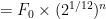Hence the general formula is $F_n = F_0 \times x^{n}$ $= F_0 \times (2^{1/12})^n$ $= F_0 \times 2^{n/12}$ .

If the starting frequency is 500 we then get the scale:

0 500.0
1 529.7
2 561.2
3 594.6
4 629.0
5 667.4
6 707.1
7 749.2
8 793.7
9 840.9
10 890.9
11 943.9

Equal temperament scale – second attempt

It’s hard to notice the difference in the first few notes, but in the end of the scale the difference gets more and more pronounced. Now we have something quite close to what’s actually used in the real world. The only difference is the starting frequency, which is usually 440 Hz, the so-called standard concert pitch. This value is somewhat arbitrary, but just for reference here’s what we get:

0 440.0
1 466.2
2 493.9
3 523.3
4 554.4
5 587.3
6 622.3
7 659.3
8 698.5
9 739.9
10 783.9
11 830.6

Chromatic scale

Fortunately it’s rather easy to implement scales once we have the theory behind us. There are two basic choices for the representation: either we work with the raw frequencies in the scale, or we work with the notes and extract the frequencies when needed. I shall go with the second option since it’s often easier to work with notes. Interestingly enough, the chromatic 12 tone scale that we just used is an example of an abelian (commutative) group with $0$ as the unit element, which means that it’s quite pleasant to work with. The basic operations that we want to perform are:

raise/2 – get the next note in the scale.
lower/2 – get the preceding note in the scale.
add/3 – add two notes in the scale.
length/1 – get the number of notes in the scale.
nth/2 – get the n:th note in the scale, starting from 0.
frequency/2 – get the associated frequency of the note.

Which is easily expressible in terms of a protocol:

:- protocol(scalep).

   :- public(raise/2).
   :- public(lower/2).
   :- public(add/3).
   :- public(nth/2).
   :- public(length/1).
   :- public(frequency/2).

:- end_protocol.

And to implement the chromatic scale is straightforward:

:- object(chromatic_scale,
        implements(scalep)).

    %A, A#, ..., G, G#.
    length(12).

    raise(N, N1) :-
        N1 is (N + 1) mod 12.

    lower(N, N1) :-
        N1 is (N - 1) mod 12.

    add(N1, N2, N3) :-
        N3 is (N1 + N2) mod 12.

    nth(I, I) :-
        % Used so that we can call nth/2 with uninstantiated
        % arguments.
        between(1, 12, I).

    %A4 to G#5.
    frequency(N, F) :-
        F is 440 * 2 ** (N/12).

:- end_object.

Extending this scale to use more than 12 elements would of course not be hard either. Just to show something different we’re also going to implement the C major scale. It contains the frequencies:

0 523.3
1 587.3
2 659.3
3 698.5
4 783.9
5 880
6 987.8

The C major scale

It’s slightly harder to implement than the chromatic scale since the distances between adjacent notes is not constant. The distance between any two adjacent notes is either a half step (the distance between two adjacent notes in the chromatic scale) or two half steps. If we then represent each note with its distance from the first note we get:

0 0
1 2
2 4
3 5
4 7
5 9
6 11

Don’t worry if these specific distances doesn’t make any sense to you. But they are not completely arbitrary; each note in C major corresponds to a white key on the piano, and is actually the only major scale that only makes use the white keys. Since we are now counting half-steps we can more or less use the same formula as in the chromatic scale for calculating frequencies.

:- object(c_major,
        implements(scalep)).

    nth(0, 0).
    nth(1, 2).
    nth(2, 4).
    nth(3, 5).
    nth(4, 7).
    nth(5, 9).
    nth(6, 11).

    raise(N, N1) :-
        nth(I1, N),
        I2 is ((I1 + 1) mod 7),
        nth(I2, N1).

    lower(N, N1) :-
        nth(I1, N),
        I2 is ((I1 - 1) mod 7),
        nth(I2, N1).

    % As far as I know, this is the only way to make sense of addition
    % in C major. Simply adding the distance from the tonic doesn't work
    % since that makes it possible to get notes outside the scale.
    add(N1, N2, N3) :-
        nth(I1, N1),
        nth(I2, N2)
        I3 is ((I1 + I2) mod 7),
        nth(I3, N3).

    % C, D, E, F, G, A, B.
    length(7).

    %C5 to B5.
    frequency(N, F) :-
        F is 440 * 2 ** ((N + 3)/12).

:- end_object.

The synthesizer

Whenever we’re going to generate music we’re going to use a specific scale in order to get a linear sequence of notes (since we don’t use chords). From the notes we get a series of frequencies. But to actually produce something that is nice to listen to we need something more. To play e.g. the standard concert pitch at 440 Hz we’re going to generate a wave with 440 oscillations per second. How we generate this wave determines how the note will be played. A sine wave will give a smooth sound while a sawtooth wave will give something reminiscent of a mechanical dentist drill. To create more complex sounds a technique known as additive synthesis can be used. We shall however not peruse this option at the moment.

Our synthesizer will take 3 input arguments: the frequency, the duration and the filter that shall be applied, and returns a list of samples in its single output argument. From the duration it’s possible to calculate how many samples that we’ll need to generate with the help of the sample rate. For example, if the duration is $0.5$ seconds and the sample rate is $22050$ the number of samples is $0.5 \times 22050$ $= 11025$ . The wave will be generated with a loop from $0$ to $Number\_Of\_Samples$ where the following operations are performed on each sample:

Divide the sample by the sample rate, so that we get the correct resolution. A high sample rate means that we’ll generate more points on the wave.
Calculate the angular frequency of the sample, i.e. $\omega = 2\pi F$ , where $F$ is the frequency.
Apply the filter. The filter should return a floating point number in $[-1, 1]$ .
Scale the sample in $[-1, 1]$ with a volume factor so that we get samples in the full sample space.

This can actually be done in rather few lines of code. Without further ado I present to you:

:- object(synthesizer).

    :- public(samples/4).
    :- public(sample_rate/1).
    :- public(bits_per_sample/1).

    :- private(filter/3).
    :- private(volume/3).
    :- private(wave//3).

    bits_per_sample(16).
    sample_rate(22050).

    samples(Frequency, Duration, Filter, Samples) :-
        sample_rate(SR),
        N is floor(SR * Duration),
        phrase(wave(N, Frequency, Filter), Samples).

    %% We could have implemented this as higher order predicates
    %% instead, but the performance loss would not have been worth it
    %% since the filter might be applied to millions of samples.
    filter(sine, Sample0, Sample) :-
        Sample is sin(Sample0).
    filter(sawtooth, Sample0, Sample) :-
        Sample is Sample0 - floor(Sample0).
    filter(triangle, Sample0, Sample) :-
        Sample is -((acos(sin(Sample0)) / pi - 0.5)*2).

    volume(M, N, V) :-
        bits_per_sample(BPS),
        V0 is (2**BPS)/2 - 1,
        %% Decrease the volume over time.
        Percent is (M/N)/2,
        V is V0*(1 - Percent).

    wave(N, Freq, F) --> wave(0, N, Freq, F).
    wave(M, N, _, _) --> {M > N}, [].
    wave(M, N, Freq, F) -->
        {M =< N,
        sample_rate(SR),
        M1 is M + 1,
        volume(M, N, V),
        X is (2*pi*Freq)*M/SR,
        filter(F, X, Sample0),
        Sample is floor(Sample0*V)},
        [word(2, little, Sample)],
        wave(M1, N, Freq, F).

:- end_object.

Putting everything together

Somehow we’ve come this far without a suitable name for the project. I’ll name it Xenakis in honor of the Greek-French music theorist, composer and architect Iannis Xenakis. You can listen to one of his most famous pieces here (warning: it’s rather frightening).

Using the components just described is not hard. First one generates a list of frequencies in a scale, that is then used as input to the synthesizer which gives a list of samples which is written to a WAV file.

:- object(xenakis).

   :- public(init/0).

   init :-
       %% N is the number of samples.
       generate_notes(Ts, N),
       wav::prepare(output, N),
       write_samples(Ts).

   %% Generate the frequencies in the C major scale. Each note has a
   %% duration of 0.5 seconds.
   generate_notes(Ts, N) :-
       Scale = c_major,
       findall(F-0.5,
               (Scale::nth(_, Note),
                Scale::frequency(Note, F)),
               Ts),
       Scale::length(L),
       synthesizer::sample_rate(SR),
       N is L*SR/2.

   %% Write the notes to 'output'.
   write_samples([]).
   write_samples([F-D|Fs]) :-
        synthesizer::samples(F, D, sine, Samples),
        wav::write_audio(output, Samples),
        write_samples(Fs).

:- end_object.

All the scales that are available on Soundcloud were of course generated using this method. We now have a good foundation for the next installment where we at last will look at methods for automatically generating note sequences.

Source code

The source code is available at https://gist.github.com/1007820.

Prolog’s Makin’ Music – Part 1

Interlude

Gather around everyone, and I’ll tell the story of how I sold my soul to the binary devil.

It all began a dark and gloomy night. I’ve had one too many to drink – coffee, that is – and found it hard to concentrate on anything else than the splashing rain. The murky light played tricks on my eyes, or so I thought. Dangling contours everywhere. The buzzing monitor didn’t help either. I stretched out my back with a loud, cracking sound and tried to suppress a yawn.

“Do you want the power to create music from thin air?”

A voice from nowhere. Surely I hadn’t had that much to drink. I held up my keyboard like a club, cursing myself for getting rid of the IBM model M keyboard in favor of an ergonomic one, and slowly turned my head in the direction of the voice. If there was an intruder, I wouldn’t go down without a fight.

“Who’s there?”, I cried.

After a long silence the voice finally answered:

“Do you want to make a deal?”

“A deal?!” I blurted out, getting rather annoyed by his impudence.

“I shall grant your computer the gift of making music. All I ask in return is that your next blog entry contains some steamy, bit-on-bit action that somehow involves the WAV format. Also, I shall need your soul for all eternity.”

Having run out of ideas, I had no choice but to accept his offer.

“Sure! Wait, no!… Who are you?”

A manic laughter followed. He vanished in a hazy puff of smoke and left. All that remained was a chilly wind and a feeling that I had somehow been cheated.

Computer generated music

Now to the point: the goal of this and the following entries will be to create computer generated music in Prolog/Logtalk. That might sound (pun not intended – I can’t help it) like a tall order, but hopefully everything will become clearer once we’ve explicated some of the concepts in music theory. The outline is as follows:

Step 1 – Generate audio.
Step 2 – Generate tones from audio.
Step 3 – Generate melodies from tones, with a suitable formalism such as a cellular automata or an L-system.

Sound as oscillations

In order to generate music we first need to understand what sound is. Wikipedia says:

Sound is a mechanical wave that is an oscillation of pressure transmitted through a solid, liquid, or gas, composed of frequencies within the range of hearing and of a level sufficiently strong to be heard, or the sensation stimulated in organs of hearing by such vibrations.

Or to put it a bit more pragmatic: a sound is a series of frequencies. Of course, this is a bit too simplistic to be useful in practice. Among other things, we need to decide whether we’re interested in mono or stereo sound, how fine-grained each frequency should be and how fast they should be played.

So we have an idea of how sound should be represented. First we decide how it should be interpreted by the listener, and then we give out the actual frequencies. As one might suspect there exists a myriad of different formats for this purpose. One of the simplest is the WAV format, which we shall use in this project.

Writing to binary files

WAV is a binary format, and thus consists of a sequence of integers of varying sizes. Hence the first step is to learn how one writes to binary files in Prolog. The bad news is that there only exists one ISO primitive for this purpose: $put\_byte/2$ , which is not sufficient since it only works for single byte, signed integers. The good news is that we can get it to do what we want with some low-level bit-fiddling. Here’s the operations that we’ll need in order to produce a fully functional WAV file:

Write 4 byte, unsigned integers in big endian format.
Write 4 byte, unsigned integers in little endian format.
Write 2 byte, unsigned integers in little endian format.
Write 2 byte, signed integers in little endian format.

It would be nice if we could handle this in a uniform way, so that the underlying details of how one should use $put\_byte/2$ can be postponed as far as possible. For this purpose we’ll introduce a data structure, $word$ , that has the format:

$word(Byte\_Count, Endian, Integer)$

where $Byte\_Count$ is either $2$ or $4$ , $Endian$ is either $big$ or $little$ , and $Integer$ is a positive or negative integer. So to represent the number $135$ in the little endian format we would use:

$word(2, little, 135)$

while the number 1350 in big endian format would represented as:

$word(4, big, 1350)$

Simple, but it might feel kind of weird to represent such a low-level concept in this way. In most imperative languages we would of course explicitly declare the data as either char, short, int and so on, but this is the best we can do in Prolog (unless we create necessary bindings for the host language and borrow some datatypes). Next, we’re going to define $write\_word/2$ that writes a word to a stream. Let’s focus on 2 byte integers for the moment. A first attempt might look like:

write_word(word(2, Endian, I), Stream) :-
    put_byte(Stream, I).

Alas, this only works for single byte integers. If we want to write 2 bytes, we need to extract the individual bytes from the integer and call $put\_byte/2$ two times. This can be done with shifting and the bitwise and-operation.

write_word(word(2, Endian, Bs), S) :-
    X1 is Bs >> 8,
    X2 is Bs /\ 0x00ff,
    (  Endian = big ->
       put_byte(S, X1),
       put_byte(S, X2)
    ;  put_byte(S, X2),
       put_byte(S, X1)
    ).

Note that we also check whether $Endian$ is $big$ , and if so output the bytes in reversed order. This works fine for positive numbers, but what about signed, negative numbers? Since $put\_byte/2$ only works with positive numbers, we need to convert the negative number into a positive number that is still negative with respect to that byte range. This is actually rather easy to do since we’re using two’s complement numbers: if the number is negative, then add a number such that the sum is the two’s complement of the absolute value of the negative number. The code will make this easier to understand:

    write_word(word(2, Endian, Bs), S) :-
        Bs >= 0,
        X1 is Bs >> 8,
        X2 is Bs /\ 0x00ff,
        (  Endian = big ->
           put_byte(S, X1),
           put_byte(S, X2)
        ;  put_byte(S, X2),
           put_byte(S, X1)
        ).
    write_word(word(2, Endian, Bs), S) :-
        Bs < 0,
        Bs1 is Bs + 0xffff,
        write_word(word(2, Endian, Bs1), S).

(Thanks to Pierpaolo Bernardi who showed me this trick on the SWI-Prolog mailing list!)
Update: Richard O’Keefe also showed a simpler solution that doesn’t need the explicit positive/negative test. It’s left as an exercise to the reader!

The code for 4 byte integers is rather similar and hence omitted.

The WAV format

Now let’s focus on WAV. All my knowledge of the format stems from a single source (click for a useful, visual diagram). A WAV file consists of:

A header containing the string “RIFF”, the remaining chunk size and the string “WAVE”.
A format subchunk containing the string “fmt” (format), the remaining chunk size, the audio format, the number of channels, the sample rate, the byte rate, the block align and the number of bits that are used for each sample.
A data subchunk that contains the string “data”, the remaining size of the subchunk and finally the actual data (the samples).

Don’t worry if some of these terms are unfamiliar or confusing. It’s not necessary to understand all the details. We begin by defining the number of samples, the number of channels, the bits per sample and the sample rate as facts:

    num_samples(100000). %This value will of course differ depending on the audio data.
    num_channels(1). %Mono.
    bits_per_sample(16). %Implies that each sample is a 16 bit, signed integer.
    sample_rate(22050).

All the other values can be derived from these parameters. For simplicity we’re going to produce a list of words that are later written with the help of $write\_word/2$ . This can be done in any number of ways, but DCG’s are fairly straightforward in this case. The RIFF chunk is first. It takes the size of the data chunk as argument since it is needed in order to produce the size of the remaining chunk.

    riff_chunk(Data_Chunk_Size) -->
        riff_string,
        chunk_size(Data_Chunk_Size),
        wave_string.

    riff_string --> [word(4, big, 0x52494646)].
    wave_string --> [word(4, big, 0x57415645)].

    chunk_size(Data_Chunk_Size) -->
        {Size is Data_Chunk_Size + 36}, % Magic constant!
        [word(4, little, Size)].

The end result will be a list of the form $[word(4, big, 0x52494646), ...]$ . The format chunk follows the same basic structure:

fmt_chunk -->
    fmt_string,
    sub_chunk1_size,
    audio_format,
    number_of_channels,
    sample_rate,
    byte_rate,
    block_align,
    bits_per_sample.

fmt_string -->  [word(4, big, 0x666d7420)]. %"fmt".

sub_chunk1_size --> [word(4, little, 16)]. %16, for PCM.

audio_format --> [word(2, little, 1)]. %PCM.

number_of_channels -->
    [word(2, little, N)],
    {num_channels(N)}.

.
.
. % And so on for all the remaining stuff.

The remaining data chunk is even simpler:

data_chunk(Data_Chunk_Size) -->
    data_string,
    [word(4, little, Data_Chunk_Size)],
    test_data.

test_data --> ... %This should generate a list of samples.

And finally, we say that a WAV file consists of a riff chunk, an fmt chunk and a data chunk:

    wav_file -->
        {num_samples(N),
         bits_per_sample(BPS),
         num_channels(Cs),
         Data_Chunk_Size is N*BPS*Cs/8},
        riff_chunk(Data_Chunk_Size),
        fmt_chunk,
        data_chunk(Data_Chunk_Size).

It is used in the following way:

    output(File) :-
        open(File, write, S, [type(binary)]),
        %Call the DCG, get a list of words as result.
        phrase(wav_file, Data),
        %Write the list of words.
        write_data(Data, S),
        close(S).

    write_data([], _).
    write_data([B|Bs], S) :-
        write_word(B, S),
        write_data(Bs, S).

As test data, we’re going to generate a 440HZ sine wave.

    sine_wave(0) --> [].
    sine_wave(N) -->
        {N > 0,
        sample_rate(SR),
        N1 is N - 1,
        %% Standard concert pitch, 440 Hz.
        Freq is 440,
        ScaleFactor is 2*pi*Freq/SR,
        %% Needed since sin(X) returns an integer in [-1, 1], which
        %% is barely (if at all) perceivable by the human ear. The
        %% constant 32767 is used since we're dealing with 16 bit,
        %% signed integers, i.e. the range of the samples is [-32768,
        %% 32767].
        VolumeFactor is 32767,
        X is ScaleFactor*N,
        Sample0 is sin(X),
        %% Floor the sample. Otherwise we would end up with a floating
        %% point number, which is not allowed.
        Sample is floor(Sample0*VolumeFactor)},
        [word(2, little, Sample)],
        sine_wave(N1).

It’s not necessary to understand all the details, but the end result is a list of 2 byte words that represent a 440 HZ sine wave. You can listen to it here.

Summary

We’re now able to write samples to WAV files. These samples can represent any tone or sound, so in theory we already have everything that’s needed to generate music. But representing a tune as millions and millions of samples is not very user-friendly and would make it more or less impossible to automatically generate anything interesting. For that we’re going to need further abstractions, and among other things define a sound bank that contains some common tones.

Source code

The source code is available at https://gist.github.com/955626.

Lindenmayer systems

Putting everything together

Source code

Share this:

Scales, scales and scales

The synthesizer

Putting everything together

Source code

Share this:

Interlude

Computer generated music

Sound as oscillations

Writing to binary files

The WAV format

Summary

Source code

Share this: